Estimate univariate and multivariate sample skewness and kurtosis in popular statistical software

For common questions, click here.

This introduces the online tool to calculate univariate/multivariate skewness and kurtosis at http://webpower.psychstat.org/models/kurtosis/

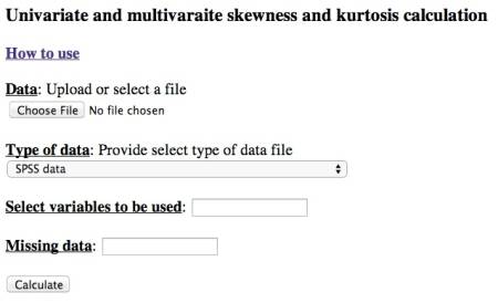
The interface of the tool looks like

The data file can be chosen by clicking the Choose File button (it might appear differently for different browsers). We DO NOT save your data file and it is deleted immediately after calculation.

The following types of data are allowed:

• SPSS data file with the extension name .sav
• SAS data file with the extension name .sas7bdat
• Excel data file with the extension name .xls or .xlsx
• CSV file (comma separated value data file) with extension name .csv
• TXT file (text file) with extension name .txt

A subset of variables can be used. To use the whole data set, leave this field blank. To select a subset of variables, provide the column numbers that separated by comma (,). For example

1, 2-5, 7-9, 11

will select variables 1, 2, 3, 4, 5, 7, 8, 9, 11

Missing data values can be provided. If multiple values are used to denote missing data, they can be separated by comma (,). For example,

-999, -888, NA

will replace all three values above to missing data.

R functions for the calculation

library(MASS)
skewkurt<-function(x, na.rm=TRUE){
    if (na.rm) x <- x[!is.na(x)]
    n <- length(x)
    skew1 <- (sum((x - mean(x))^3)/n)/(sum((x - mean(x))^2)/n)^(3/2)
    skew2 <- n/((n-1)*(n-2))*sum((x - mean(x))^3)/(sd(x))^3
    skew.se <- sqrt(6*n*(n-1) / ((n-2)*(n+1)*(n+3)))

    temp<- sum((x - mean(x))^4)/(sum((x - mean(x))^2)^2)
    kurt1 <- n * temp -3     
    kurt2 <- n*(n+1)*(n-1)/((n-2)*(n-3))*temp - 3*(n-1)^2/((n-2)*(n-3))
    kurt.se <- sqrt(4*(n^2-1)*skew.se^2 / ((n-3)*(n+5)))
    list(skew1=skew1, skew2=skew2, skew.se=skew.se, kurt1=kurt1, kurt2=kurt2, kurt.se=kurt.se)
}


multi.skewkurt<-function (x, na.rm = TRUE){
    x <- as.matrix(x)
    if (na.rm) 
        x <- na.omit(x)
    n <- dim(x)[1]
    p <- dim(x)[2]
    x <- scale(x, scale = FALSE)
    S <- cov(x)*(n-1)/n
    #S.inv <- solve(S)
    S.inv <- ginv(S)
	D <- x %*% S.inv %*% t(x)
    b1p <- sum(D^3)/n^2
    b2p <- tr(D^2)/n
    chi.df <- p * (p + 1) * (p + 2)/6
    k <- (p + 1) * (n + 1) * (n + 3)/(n * ((n + 1) * (p + 1) - 
        6))
    small.skew <- n * k * b1p/6
    M.skew <- n * b1p/6
    M.kurt <- (b2p - p * (p + 2)) * sqrt(n/(8 * p * (p + 2)))
    p.skew <- 1 - pchisq(M.skew, chi.df)
    p.small <- 1 - pchisq(small.skew, chi.df)
    p.kurt <- 2 * (1 - pnorm(abs(M.kurt)))

    results <- list(n.obs = n, n.var = p, b1p = b1p, b2p = b2p, 
        skew = M.skew, small.skew = small.skew, p.skew = p.skew, 
        p.small = p.small, kurtosis = M.kurt, p.kurt = p.kurt)
    return(results)
}

mardia<-function(x, na.rm=TRUE){
	if (na.rm) 
	x <- na.omit(x)
	n <- dim(x)[1]
	p <- dim(x)[2]
	
	uni <- function(x){
		n <- length(x)
		xbar <- mean(x)
		m2 <- sum((x-xbar)^2)/n
		m3 <- sum((x-xbar)^3)/n
		m4 <- sum((x-xbar)^4)/n

		skewness <- sqrt(n*(n-1))/(n-2)*m3/m2^1.5
		kurtosis <- (n-1)/((n-2)*(n-3))*((n+1)*(m4/m2^2-3)+6)
		
		skew.se <- sqrt(6*n*(n-1) / ((n-2)*(n+1)*(n+3)))
		kurt.se <- sqrt(4*(n^2-1)*skew.se^2 / ((n-3)*(n+5)))
		c(skewness, skew.se=skew.se, kurtosis, kurt.se)
	}
	
	univariate <- apply(x, 2, uni)
	rownames(univariate) <- c('Skewness', 'SE_skew', 'Kurtosis', 'SE_kurt')
	
	x <- scale(x, scale = FALSE)
	S <- cov(x)*(n-1)/n
	S.inv <- ginv(S)
	D <- x %*% S.inv %*% t(x)
	b1p <- sum(D^3)/n^2
	b2p <- sum(diag(D^2))/n
	chi.df <- p * (p + 1) * (p + 2)/6
	k <- (p + 1) * (n + 1) * (n + 3)/(n * ((n + 1) * (p + 1) - 6))
	small.skew <- n * k * b1p/6
	M.skew <- n * b1p/6
	M.kurt <- (b2p - p * (p + 2)) * sqrt(n/(8 * p * (p + 2)))
	p.skew <- 1 - pchisq(M.skew, chi.df)
	p.small <- 1 - pchisq(small.skew, chi.df)
	p.kurt <- 2 * (1 - pnorm(abs(M.kurt)))
	
	multivariate <- rbind(c(b1p, M.skew, p.skew), c(b2p, M.kurt, p.kurt))
	rownames(multivariate) <- c('Skewness', 'Kurtosis')
	colnames(multivariate) <- c('b', 'z', 'p-value')

	results <- list(n.obs = n, n.var = p, univariate = univariate, multivariate=multivariate)
	
	cat('Sample size: ', n, "\n")
	cat('Number of variables: ', p, "\n\n")
	
	cat("Univariate skewness and kurtosis\n")
	print(t(univariate))
	
	cat("\nMardia's multivariate skewness and kurtosis\n")
	print(multivariate)
	cat("\n")
	
	invisible(results)
}

An SPSS macro developed by Dr. Lawrence T. DeCarlo needs to be used. We have edited this macro to get the skewness and kurtosis only.

First, download the macro (right click here to download) to your computer under a folder such as c:\Users\johnny\.

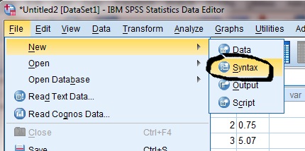
Second, open a script editor within SPSS

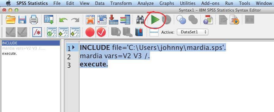
Third, in the script editor, type the following

INCLUDE file='C:\Users\johnny\mardia.sps'.
mardia vars=V2 V3 /.
execute.

Note that you will need to change the folder to the SPSS macro file you just downloaded. Also, the vars to use to calculate the skewness and kurtosis should be changed from V2 V3 to your variables.

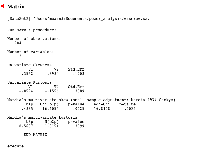
Finally, the output is shown like

A SAS macro can be used to calculate multivariate skewness and kurtosis. We have edited this macro to get the skewness and kurtosis only.

First, download the macro to your computer, e.g., to C:\Users\johnny\. right click here to download the macro

Second, in the sas script editor, type

%inc "C:\Users\johnny\mardia.sas";
%mardia(data=testdataset, var=V2 V3)

The first line provides the sas macro file location. In the second, one needs to specify the data and variables to use.

An example is shown below

data cork;
           input n e s w @@;
           datalines;
         72 66 76 77   91 79 100 75
         60 53 66 63   56 68 47 50
         56 57 64 58   79 65 70 61
         41 29 36 38   81 80 68 58
         32 32 35 36   78 55 67 60
         30 35 34 26   46 38 37 38
         39 39 31 27   39 35 34 37
         42 43 31 25   32 30 30 32
         37 40 31 25   60 50 67 54
         33 29 27 36   35 37 48 39
         32 30 34 28   39 36 39 31
         63 45 74 63   50 34 37 40
         54 46 60 52   43 37 39 50
         47 51 52 43   48 54 57 43
         ;

         %inc "C:\Users\johnny\mardia.sas";
         %mardia(data=cork, var=n e s w)

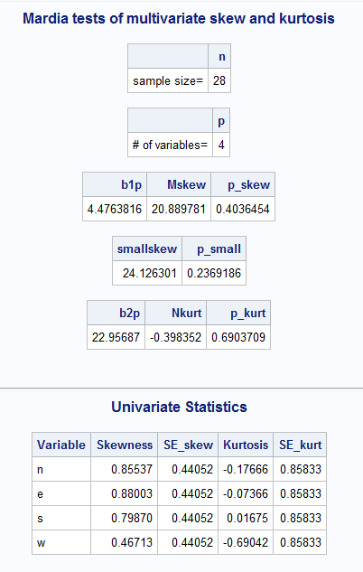
The sample output looks like this

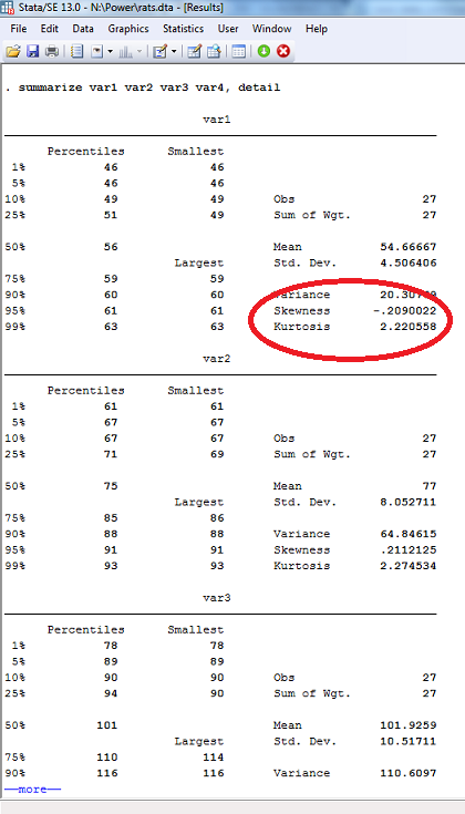
Univariate skewness and kurtosis can be calculated in STATA along with other descriptive statistics by adding detail as an option to the summarize command:

summarize var1 var2 var3 var4, detail

Just change var1, var2, etc. to the variables of interest in your data set. Skewness and kurtosis will appear in the lower right corner of each variable's output

Multivariate skewness and kurtosis can then be calculated using the following syntax:

mvtest normality var1 var2 var3 var4, stats(skewness kurtosis)

Again, specify the appropriate variable names. The sample output will appear as

• Yes! If you send us the data, we can do the calculation by ourselves and delete the data from our computer once it is done.

• We are interested in the skewness and kurtosis of all the continuous variables (including ordinal ones such as likert scale variables) you have used in the data analysis of your paper. Therefore, do not include categorical, binomial, or proportional data, etc. Note that this means to not include ID, condition #, or other such variables in your calculations. If you have used composite scores such as mean or sum scores, please calculate skewness and kurtosis for them instead of the item scores.

• If items have been reverse-coded, please make sure to only include one or the other.

• If there are no suitable variables from your paper then please ignore our email. Nevertheless, we appreciate your interest in our study!

• Please calculate skewness and kurtosis separately for each study. This is especially important for multivariate skewness and kurtosis as we only want those measures of a group of variables used together in the same analysis.

• Convert your data to csv format and use the online calculator. Please let us know if you run into trouble.

• We are interested in the skewness/kurtosis of all papers published in Psychological Science and the American Educational Research Journal in the past 5 years.